Lesson 6 Projections

Accurately projecting the Earth’s surface onto a map is a challenging task. There are many concepts to keep in mind when trying to choose a map projection.

This lesson discusses the different types of map projections, their parameters and properties, and the criteria for choosing an appropriate projection.

Upon completion of this lesson, you should be able to:

• Describe the basic principles of map projections
• Distinguish between the major types of map projections and their characteristics

6.1 Introduction

Figure 6.1: Video (0:48) Projections - simply explained.

It might appear sufficient to limit our work with spatial data to a geographic coordinate system. After all, the location of each point on the Earth’s surface can be clearly described in this way. However, a closer examination reveals that defining each point on Earth is not indeed possible. This brings us to the topic of cartographic projections. The problem, of how to map the three-dimensional curved surface of the Earth occurs in all common ways of visualising spatial data - both, while presenting it on a screen and while producing paper maps. The only exception is the local scale representation of the Earth on a globe.

It is commonly understood that a certain amount of original information is lost when using projections, resulting in inaccuracy. Different approaches (in projections) are used depending on the purpose of the presentation and the location and size of the area being represented. Therefore, the knowledge of common projections and their suitability for different situations is one of the main and necessary prerequisites for working with GIS.

6.2 Types of Projections

Figure 6.2: Projection with light: Move your mouse over the image to turn the light on and off!

Over time, different methods have been developed to project the coordinate systems of the curved surface of the Earth onto a planar surface (plane). This process can simply be imagined as the result of projecting the Earth’s surface on a screen using a light source, as shown in Figure 6.2.

However, the projected surface of the Earth often does not correspond to a flat projection plane but is instead wrapped around the Earth in the form of a cylinder or cone. Accordingly, the resulting geometric structure can be categorised into four types:

• Azimuthal projections
• Cylindrical projections
• Conic projections
• Pseudo- and other projections

6.2.1 Azimuthal projections

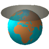
Figure 6.3: Azimuthal projection.

Azimuthal projections are also called planar projections (Figure 6.3). In an azimuthal projection, the graticule of the Earth is transferred to a plane that normally lies at the North or the South pole (instead of lying along a tangential plane). The resulting contact of the graticule to the pole shows concentric circles of latitude and radial shapes – meridians – emanating from the centre. The angles between the meridians (azimuth) in the projection are identical to the original ones on Earth.

Azimuthal projections are rarely used to represent the entire Earth. Instead, they are suitable for the representation of individual parts or hemispheres.

6.2.2 Cylindrical projections

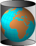
Figure 6.4: Cylindrical projection.

These projections result from wrapping a cylinder around the Earth, as shown in Figure 6.4, which is then unrolled into a plane. In its normal position, in which the axis of the cylinder and the rotation axis of the Earth coincide, the cylinder touches the Earth at the equator. In this case, the resulting image of the projected latitudes and longitudes are parallel lines that intersect each other at right angles. Cylindrical projections are used to represent the whole Earth, as well as for continental scale depiction of smaller areas. For example, the official base maps of Austria, Germany, and Switzerland are based on cylindrical projections.

6.2.3 Conical projection

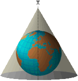
Figure 6.5: Conical projection.

In Figure 6.5, the surface used to construct a projection is a cone that touches a globe along any small circle or the cone cutting through the respective globe. The cone is then cut along one of the lines from its apex to the edge resulting in a projection plane with the meridians converging in the apex and curved parallels. All lines intersect at right angles (as in the azimuthal and cylindrical projections).

Conic projections are mainly used for medium to local scale areas. They are especially suitable for mid-latitude regions with a large east-west extension (e.g., 1:500,000 overview map of Austria, outline map of the United States).

6.2.4 Pseudo- and other projections

As shown in Figure 6.6, these projections can hardly be described using the “light bulb illumination” analogy because they do not refer to any regular geometric projecting surface. For example, such a pseudo projection may look like a cylindrical one with its lines at their ends curved inwards.

Pseudo projections are mostly used for mapping the entire surface of the Earth (planisphere). Given that most GIS applications operate in larger scale areas, the pseudo projections play a less important role in the context of GIS.

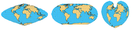
Figure 6.6: Pseudo projections.

6.2.5 Map projection aspect

The map projection aspect refers to the point or line(s) of tangency on the projection surface. In theory, it can touch or intersect anywhere on the projection surface. The quality of a projection is best where the projection surface touches the Earth surface. For example, an azimuthal projection where the projection plane touches the Earth at or near the north pole results in significantly better projections for the close-to-polar areas than the equatorial regions. In contrast, a cylindrical projection tangential to the equator is better for the equatorial areas than for a polar region.

How is it that highly accurate, large-scale maps are based on a cylindrical projection? E.g., in Europe, we are quite far away from the equator. To project any (small) part of the Earth’s surface in high quality we change the position of the (geometrical) projection body relative to the Earth. For example, with a horizontal cylinder, even areas outside the equatorial zone are represented with sufficient accuracy. We distinguish between the following three aspects of projection:

• Normal aspect:
  The axis of the projection body corresponds to the Earth’s axis.
• Transverse aspect:
  The axis of the projection body is perpendicular to the axis of the Earth.
• Oblique aspect:
  The axis of the projection body is tilted to the Earth’s axis.

As shown in Figure 6.7, the choice of a map projection aspect results in different presentations of the graticule and distribution of land masses. The distortion properties of any given projection surface, however, remain unchanged when the aspect is changed.

Figure 6.7: Projection aspects.

6.2.6 Tangents vs. secants

As you already know, there are three types of projection surfaces: a cone, a cylinder, or a plane. Imagine the Earth wrapped up in one of these projection (developable) surfaces. The quality aspect of a true projection depends on whether this developable surface just touches (= tangent case) the Earth’s surface or intersects it (= secant case).

The resulting standard parallel is the line of latitude where the projection surface touches the globe. As shown in Figure 6.8, a tangent conic or cylindrical projection has one standard parallel, while a secant conic or cylindrical projection has two. The standard parallel has no distortion. The distortion, however, increases towards the middle and the edges.

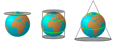
Figure 6.8: Different standard parallels.

Compared to the tangent approach, the secant approach allows almost doubling the area to be projected while at the same time preserving the quality of the projection. Here is an example: Before the year 2000, for the base map of Austria in 1:500,000 a transverse cylindrical projection (Gauss-Krüger) was used, which covers a 3° zone pro central meridian. Since 2000, a transverse cylindrical projection (Universal Transverse Mercator – UTM) is used, which covers a 6° zone pro central meridian while retaining the same quality characteristics.

Figure 6.9: Tangent and secant cases and the degree of distortion.

6.2.7 Effects of light source on the projection plane

So far, we assumed the light source used for the projection to be at the centre of the Earth. Changing the position of this light source can result in different perspectives in the projection, i.e., different mappings of the graticule onto the projection surface. The light source can be positioned in three locations: the centre of the Earth, opposite sides of the Earth, and infinite location in space (Figure 6.10).

Conical and cylindrical projections usually use a light source emanating from the centre of the Earth. In azimuthal (planar) projections, the effects of using light sources in different positions can be seen clearly, especially on polar projections. You can see that in the Gnomonic projection, most of the latitudes/parallels are not visible at all, but great circles are represented as straight lines. Orthographic projection, on the other hand, almost resembles the view that a geographer would expect when seeing Earth from space.

Figure 6.10: Light source and projection plane.

The analogy to positioning a light source applies well to the example in Figure 6.10 (true perspective projection); though, for many other projections this does not apply. In those cases, it is necessary to allow the existence of curved projection rays and account for them in the underlying mathematical algorithms.

6.3 Projection Parameters

Projections are used to map the entire world as well as to map a specific area such as a continent, a war zone, etc. In any of these cases you want to have a projection that is just right (exact); that is, you want to select a projection for which distortions are known and kept to a minimum. This can be achieved by the selection of appropriate parameters. Projection parameters are a series of values that define a particular projection that tell how the projection is related to the Earth. Projection parameters may indicate the point of tangency or the lines where a secant surface intersects the Earth. They also define the spheroid used to create the projection and any other information necessary to identify the projection.

Projection parameters are of two types: angular and linear (Kimerling et al. 2016).

6.3.1 Angular parameters

Central Meridian/Longitude of Origin is a geographic longitude that refers to the origin of the projection. Such a meridian lies at the centre of the resulting map sheet. The origin of the projection is also the origin for the x and y coordinates in the projection. In Figure 6.11 the 0° meridian is used as origin.

Figure 6.11: Longitude of Origin.

Latitude of Origin / Reference Latitude is a latitude that defines the origin of a map projection. The intersection of the latitude and longitude of origin is the origin for map projections (x, y). A change of latitude of origin does not affect the mapped content; only the origin of the y-coordinate values changes accordingly. An exception here are azimuthal projections: the change of the latitude of origin changes the location of the projection surface and with that significantly influences the resulting map content (map body). As shown in Figure 6.12, the parameter value of 45° indicates the latitude of origin = 45°N.

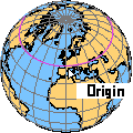
Figure 6.12: Latitude of Origin.

Standard Parallel / Latitude of True Scale is the line of latitude in a conic or cylindrical projection in normal aspect where the projection surface touches the globe. A tangent conic or cylindrical projection has one standard parallel, while a secant conic or cylindrical projection has two. At the standard parallel, the projection shows no distortion. See Figure 6.13, for a visualisation of a conic projection with two standard parallels.

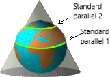
Figure 6.13: Standard Parallels.

Latitude of Centre / Central Parallel – Similar to the central meridian (except for latitudes, of course), this latitude is the middle latitude of a projection. Its intersection with the central meridian is the origin of a map projection point. It is used mainly with projections that have single points of zero distortion (like Gnomonic and Orthographic projections). Note: While the latitude of origin does not have to lie in the centre, the central parallel does.

6.3.2 Linear parameters

6.3.2.1 False easting / false northing (false x, false y)

Projected coordinates (i.e., x, y coordinates) have positive values for some locations and negative for the others. This depends on where the x- and y-axes intersect. On published maps that use x, y coordinates as reference, it is common practice to have positive values for all coordinates. For example, if your area of interest is favourably located, no action is required at your end. You can influence it by the choice of the central meridian and latitude of origin. A convenient way is the use of false easting and false northing values: These are two big numbers – constants – that are added to each x- and y-coordinate, respectively. The selected constants are big enough to make sure that all the coordinate values in your area of interest have a positive value.

Example: The coordinate system of Austria for ÖK 1:50,000 has its origin in the intersection of each of the central meridians with the equator; thus, the y-value corresponds to a distance from equator. The y values in Austria range from ca. 5,130,000 to 5,430,000 meter. In order to speed up writing, the false northing value of -5,000,000 is introduced; so, from each y the value 5,000,000m is subtracted resulting in values with considerably fewer digits.

6.3.2.2 Scale (reduction) factor

A map scale is a ratio between a distance on a map and the respective distance in reality. Due to stretching and shrinking that occurs while transforming an ellipsoidal Earth surface onto a plane, the map scale will vary across the mapped area (i.e., across the map). We, therefore, distinguish between 2 types of scales (Kimerling et al. 2016):

The actual (true) scale is the one we can measure at any point on the map. It varies from location to location and is a direct consequence of the geometrical distortion from flattening the Earth.

The principal scale is the desired scale of a map, i.e., the one we reduce a generating globe to. It is stated on a map in form of a text or a scale bar. This scale is true only at selected points or along specific lines, i.e., points or lines of tangency. The relationship between the actual and the principal scale is described as the ratio of the true map scale to the stated map scale at a particular location and is called the scale factor (SF):

SF = actual scale / principal scale
SF = 1 for a line of true scale (also called unity)
SF > 1 the actual scale is larger than the principal scale
SF < 1 the actual scale is smaller than the principal scale

E.g., SF = 1.15 on a regional map means that the actual scale is 15% larger than the principal scale. SF = 2 means the distance is twice as long whereas SF = 0.5 means the distance is half of the actual distance.

Scale distortion is related to the size of the mapping area: the smaller the area to be mapped, the less the scale distortion. Following this general rule, for continental scale maps SF should only slightly vary from 1.0.
The choice of a scale factor influences (indirectly) the distance between the secant lines. A commonly used value SF = 0.9996, for example, results in secant lines at a distance of ca. 360km (180km on each side from a central meridian). This way we can balance the distortion within the area of interest.
Remember the Orange-Video in Figure 6.1!

6.4 Properties of Projections

Geometric distortions are inevitable when mapping spherical surfaces. Different projections are characterised by the fact that they can preserve some geometrical properties at the expense of other geometric properties. For example, if the relative sizes of regions on Earth were preserved everywhere on a map, their shapes would be deformed to a lesser or greater extent.

Since no single projection can preserve all the geometric properties, the choice of a suitable projection is made according to the importance of certain criteria in an area / project / application. Compromises must be made between the preserving properties. This becomes more important with the increasing distance from a point or line of tangency, i.e., the larger the size of the mapping area.

Map projections can have the following geometric properties:

• Equidistant – preserves distance. A distance measured on a map and multiplied by the scale factor results in the true distance in nature. Usually, this property is preserved only along tangent or secant lines or in a specific direction.

• Equal area – preserves the size of a region. A measurement of the size of a region (area) on a map corresponds to the size of that region in reality, considering the respective scale.

• Conformal – preserves angles, locally. A specific, local angle on a map is consistent with the respective, local angle on the Earth’s surface. This property leads to local (!) preservation of shapes (i.e., correct form of a shape).

• True direction – preserves global directions. A specific direction on a map at any point should correspond to the actual direction in which the point is located.

6.5 Equidistant Projections

“If you want to determine the distance between two points, then take the map, measure the distance between these points using a ruler and multiply the result with the scale factor of the map…”. That’s what most of us learned in geography lessons. In many cases this task is not so easy.

Look at the following brainteaser in Figure 6.14:
The distance between points A and C and between C and D is about 10,000 kilometres respectively.
What is the distance between A and D?

Figure 6.14: Move your mouse over the image to get the solution.

Generally, it is impossible to create a map that has true-to-scale distances in all directions and between all points. We, therefore, speak of partially equidistant projections.

6.5.1 Azimuthal Equidistant Projection

Unlike other equidistant projections where “true distance” is restricted to certain directions (azimuthal equidistant), in an equidistant azimuthal projection, true (= spherical) distances can be determined in all directions. This, however, holds true for a single point, i.e., the tangent point. For this reason, this projection must be specifically tailored for each point from which you want to measure spherical distances.

The projection shown in Figures 6.15 and 6.16 is approximately the equidistant projection of Salzburg (red dot roughly in the middle). Equidistant azimuthal projections can represent not only a hemisphere, but the entire world. However, the shape-related distortions increase rapidly towards the edges. The constant latitude intervals make it clear that the length of the meridians in this situation remains the same.

In addition to the equidistant property, this projection also preserves direction but only in its origin, i.e., the point of tangency; it is, therefore, possible to determine the cardinal direction in which a point lies compared to the origin. Due to this property, all great circles passing through the origin are represented by the projection as straight lines. The property of true direction is particularly important for navigation purposes. So, referring to the figures below, you can not only find out how far the (direct) flight route between Salzburg and any other place is, but also about areas / places that lie on the flight path. This projection is used in a wide range of applications like navigation, radio relay, and also in the representation of polar regions.

Figure 6.15: Hemisphere.

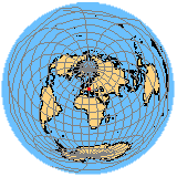
Figure 6.16: Whole Earth.

A popular example for azimuthal equidistant projections is the logo of the UN as shown in Figure 6.17 and Figure 6.18:

“The logo of the United Nations is a map of the world representing an azimuthal equidistant projection centred on the North Pole, inscribed in a wreath consisting of crossed conventionalized branches of the olive tree,… The projection of the map extends to 60 degrees south of latitude, and includes five concentric circles.” (United Nations, 1946).

Figure 6.17: Logo of the United Nations. (Source: AdobeStock)

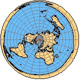
Figure 6.18: Polar projection as in the UN logo.

6.5.2 Equidistant cylindrical projection

The equidistant cylindrical projection (equidistant cylindrical, cylindrical equirectangular, plane chart) only has true distance along the equator and the meridians (Figure 6.19). For distance measurements with an east or west component, the scale increases rapidly when moving from the equator towards the poles. The maximum deviation in horizontal distances can be seen at the poles, which are shown on the map as lines with the length of the equator. An equidistant cylindrical projection with the line of tangency at the equator and with the origin at 0.0 is also called “Plate Carree”. The degrees of latitude and longitude are presented as if they were Cartesian coordinates. This simple planar representation of spherical coordinates is used in most GI-Systems as standard representation of unprojected spatial data.

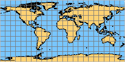
Figure 6.19: Plate Caree.

6.5.3 Digression: The compass problem

Consider this:

A rocket that is launched from Salzburg, Austria, heads east and needs to fly in a straight line around the world.

Before you continue reading, think about the countries it would cross in its flight path? If you thought the rocket flies over China and the U.S.A, you are mistaken. In reality, the rocket crosses the equator near Sumatra, flies over Australia, enters the northern hemisphere near Colombia and finally returns to Salzburg. At each point of this path, the rocket is exactly east (or west) of the starting point (Salzburg, Austria). This is because the true east direction is determined by following the great circle that intersects the reference meridian at a right angle. Now, a completely different situation arises if the rocket uses a compass to find east and steers itself in the direction pointed by the compass. The flight path using a compass will resemble a latitude / parallel circle crossing China and the United States. Although the rocket is now flying east, it no longer refers to its starting point (Austria). Instead, it uses the last meridian it flew over as a reference to find which direction is east. From Austria, it would seem that the rocket constantly changes its direction according to the direction pointed by the compass. Therefore, a directional antenna attached to the rocket would have to be adjusted/aligned continuously.

In case 1 the rocket flies along a great circle and in case 2, it moves along a rhumb line (see Lesson on Coordinate Systems to refresh your memory on a rhumb line). In case 1, the cardinal direction in which the rocket is located to the starting point is constant. The (course) angle changes constantly but with respect to the north.

The situation is exactly the opposite in case 2: The course changes continuously in the direction of movement by always steering slightly to the left and, therefore, the cardinal direction in which it is located also changes with respect to the starting point. However, the respective (course) angle - the angle between the last reference meridian that gets crossed and the east direction pointed to by the compass - with respect to the north remains constant.

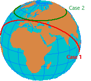
Figure 6.20: Two cases of the flight path of a rocket.

In Figure 6.20, you can see that there is a significant difference between the supposed cardinal direction in which a destination point lies and the cardinal direction that needs to be retained to reach that point. In practice, the kind of application determines which of the two cases is needed. For example, true direction is important in the field of transmitting radio waves or for some military applications like long range unguided missiles. The second case requires navigation with a compass from A to B.

Consequently, a design of a grid will differ accordingly to meet various requirements: To determine the cardinal direction in which a particular point lies, you need a projection that has true direction (i.e., is zenithal) and in which great circles are projected to straight lines. However, to determine the course angle, which is to be followed to reach a destination, you need a conformal projection in which rhumb lines become straight lines.

6.6 Equal Area Projections (preserve area)

Equal area projections preserve the relative size of regions on the entire map, and they have the property of equivalence. Due to demands of equivalence, the scale factor can only be the same along one or two lines or from a maximum of two points. Scale factors and angles around all other points will be deformed; it is, therefore, impossible to have a projection that is equal area and conformal at the same time. It is only possible on the globe. Shape, distance, and direction are most distorted towards the edges of the map.

The equivalence property is mostly needed in middle- and local scale representation. The property of equal area is always important when comparing an area or density between regions. This is true especially for world maps that need to communicate the spatial distribution of attributes like population density, literacy, poverty, and other human-related statistics. In such cases, a choice of an inappropriate projection may lead to a completely wrong interpretation of the situation. The fact that maps can “lie” by distorting represented surfaces has often been exploited for propaganda purposes.

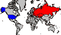
Figure 6.21: Cold War Map.

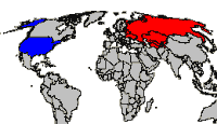
Figure 6.22: Mollweide Equal-Area Map.

During the Cold War, U.S. cartographers deliberately used Mercator projection to create a world map (Figure 6.21) and highlighted the U.S.S.R in red to make it appear larger, closer, and more threatening. Figure 6.22 shows a world map in the equal-area Mollweide projection. Note the difference in the areas of Greenland and Africa.

6.6.1 Exercise: The true size

The app the true size.com (created by James Talmage and Damon Maneice) illustrates the effect of the widely used Mercator projection on area sizes in that the countries near the poles appear bigger and those near the equator appear smaller than their true size. Use this app to explore the area sizes of the world countries.

Compare the true size of your home country to other countries of your choice!

6.6.2 Lambert equal-area azimuthal projection

This equal area azimuthal projection (Figure 6.23) was presented by Johann Heinrich Lambert, in 1772. Around the point of tangency, this projection is very similar to the azimuthal equidistant projection discussed above. Towards the edges of a map, i.e., in the areas of the other hemisphere, the distance distortion increases rapidly to preserve relative sizes of regions. Consequently, Antarctica is represented as a thin ring. The Lambert equal-area azimuthal projection is mainly used to represent small regions (regions with a compact form).

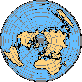
Figure 6.23: Lambert equal-area azimuthal.

6.6.3 Albers equal-area conic projection

The construction of Albers equal-area conic projection (Figure 6.24) can be imagined as if light rays emanating from the Earth’s surface strike the projection cone at a right angle. This projection is equidistant along the standard parallels; Geometric distortions (i.e., shape distortions) found near the standard parallels are within tolerable limits. Albers equal-area conic projection is suitable for thematic maps with an explicit East-West extent as the projection compresses North-South areas between each parallel to compensate for East-West stretching.

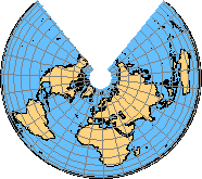
Figure 6.24: Albers equal-area conic.

6.6.4 Eckert IV

This projection is similar to the Mollweide projection for the representation of thematic content at a global scale (Figure 6.25).

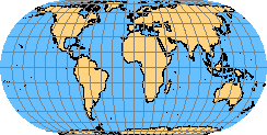
Figure 6.25: Eckert IV.

6.7 Conformal Projections

A conformal projection preserves angles while locally preserving shape at the same time; the term conformal means “correct form or shape” (Kimerling et al. 2016). Although the scale varies in a conformal projection, distance distortions in any point are equal in all directions. Conformal projections are particularly important in the field of navigation as they represent rhumb lines as the straight lines. (Rhumb lines are straight line segments that preserve the angles with the meridians.)

With a conformal map, one cannot determine the direction in which a certain point lies; but we can determine the azimuth of this point which will get us to that point (revisit the The Compass Problem). As already known from the lesson on coordinate systems, the travelled distance rarely corresponds to the shortest path. The latter runs along a great circle and requires a constant correction of the direction.

6.7.1 Mercator projection

The Flemish cartographer Gerhard Kremer (Figure 6.26) published an atlas in 1569, under his latinised name Gerardus Mercator.

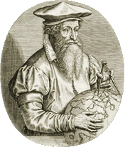
Figure 6.26: Gerardus Mercator (1512-1594).

The Mercator projection is a conformal, cylindrical projection that provided a considerable ease in navigation for generations of sailors and still is one of the most important projections. The Mercator projection in its normal position represents almost the entire Earth. Areas above the 80° - 85° latitudes are usually not mapped anymore because the distortion increases greatly in the direction of the poles, and these lie in infinity. The area exaggeration in Europe, Russia, and North America provides an incorrect impression of the size of the respective land masses (Figure 6.27). Explore this phenomenon in the Engaging Data web-application. The usefulness of the Mercator projection is limited to non-polar areas.

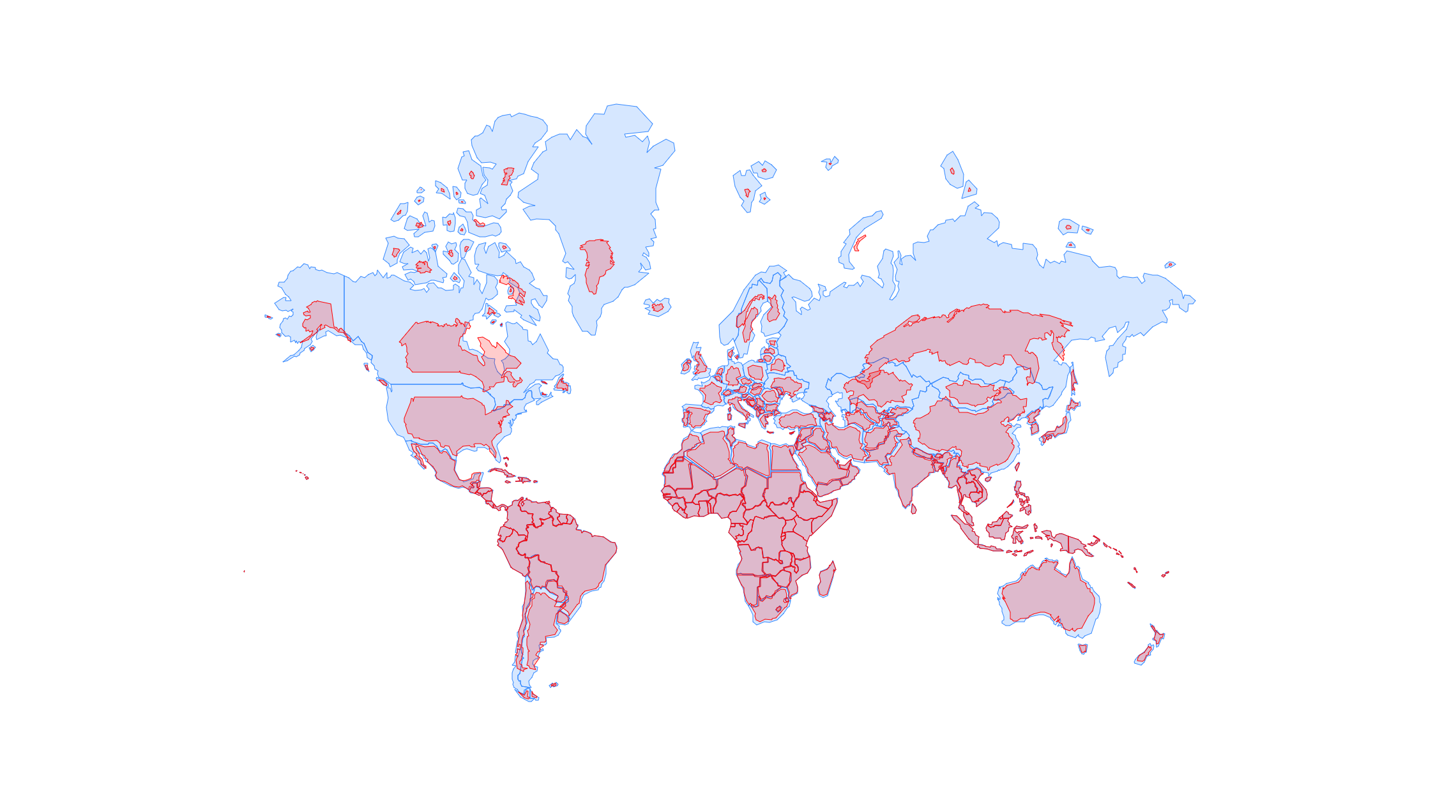
Figure 6.27: Real country sizes shown compared to a Mercator projection (image source: engaging-data.com).

Figure 6.27 nicely demonstrates that the Mercator projection is absolutely unsuitable for maps of the entire Earth, because of its extreme distortions close to the poles. To overcome this problem, the transverse Mercator projection is used today. In contrast to the standard Mercator projection, that wraps around the equator, the transverse Mercator projection is turned by 90° and wraps around a meridian, as you can see in (Figure 6.28):

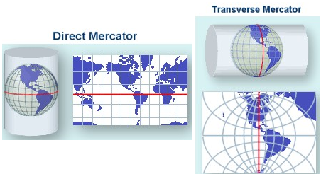
Figure 6.28: Standard Mercator projection versus transverse Mercator projection.

The most prominent use of the transverse Mercator projection is the world-wide system of the Universal Transverse Mercator (UTM). UTM divides the Earth into 60 zones, each of which is 6° wide. Further examples of transverse Mercator projections are the national mapping systems of Austria (ÖK 1:50,000) and Germany (TK 1:25,000).

6.7.2 Lambert conformal conic projection

This projection is named after the Swiss mathematician Johannes Lambert (Figure 6.29), who proposed not less than six projection systems. Three of them are still widely used today: the Lambert conformal conic projection, the Lambert azimuthal equal area projection, and the transverse Mercator projection.

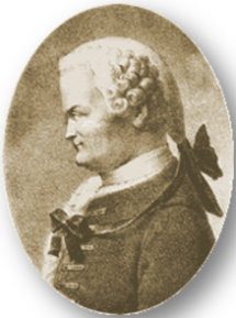
Figure 6.29: Johann Lambert (1728-1777).

Like all conic projections the Lambert conformal conic projection (Figure 6.30) is used especially for maps of regions with a pronounced East-West extent. Naturally, this projection focuses on preserving angle and/or shape. For example, the shapes of the states are correctly reproduced, but at the cost of proportion of areas of individual states. In comparison, Albers equal-area conic projection preserves the true area but distorts the shape. Such differences are increasingly obvious the farther one moves away from the standard parallels (in both cases the 43° and 62° degree of latitude).

The Lambert conformal conic projection is used in the official cartography of Austria and Germany for nation-wide maps. It is also used as the basis of the system zones in the east-west lying states of the United States like Oregon and Wisconsin. One of the major uses of this projection are aeronautical charts because navigators and pilots prefer navigational charts that preserve shapes and directions locally (Kimerling et al. 2016).

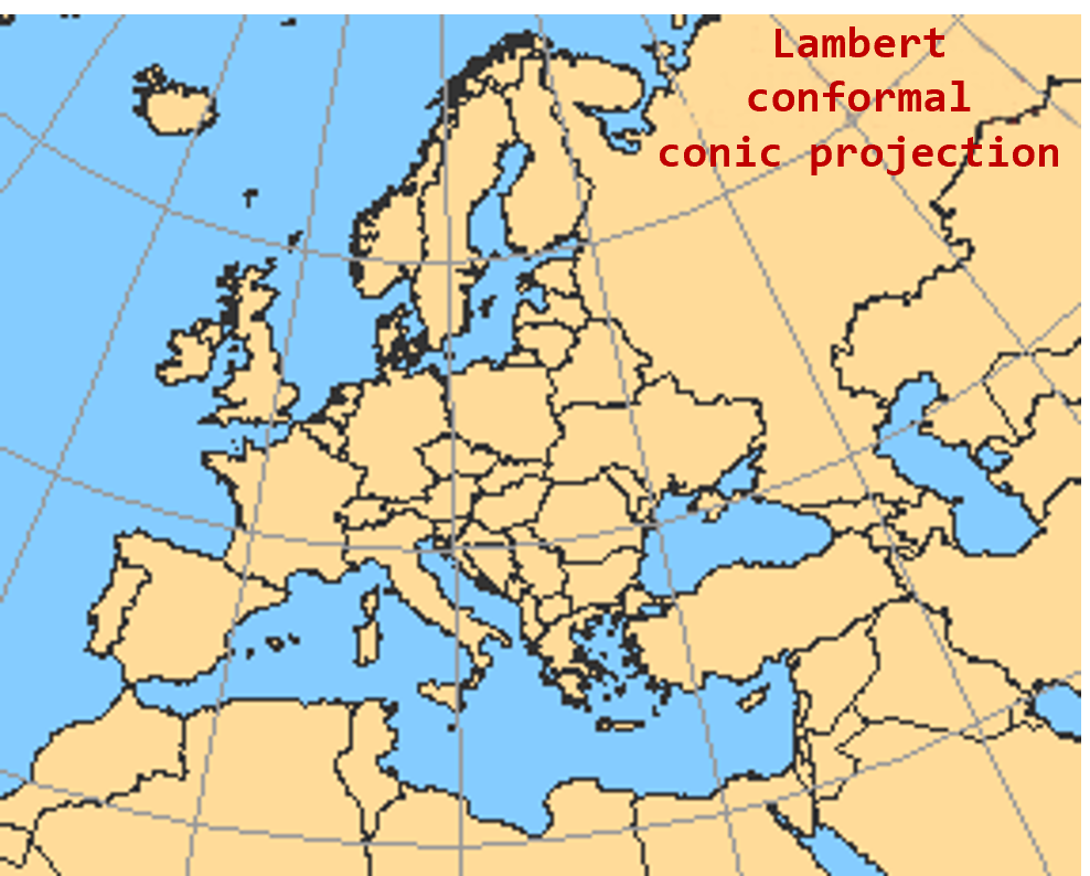
Figure 6.30: Lambert projection.

6.8 True direction projections

True direction projections preserve directions globally, unlike the conformal projections that preserve angles locally. These projections are sometimes also referred to as azimuthal projections because one cannot find the true direction in all areas of a map but only in the point of tangency (i.e., azimuthal or planar projections).

In azimuthal maps, great circles running through the point of tangency are represented as straight lines. This allows us to determine the direction between two points, i.e., the most direct way (great circle segment) from A to B. In the gnomonic projection, which preserves direction, the great circles are represented as straight lines running through the point of tangency.

If the difference between true direction and true angle property is still unclear, have a look at the problem of the compass. True direction projections are applied wherever shortest paths or straight-line spreading are of importance. In the past, ship routes used to be first determined as straight lines on a true direction map and then transferred to a conformal map. From the latter map, the necessary corrections to be made while navigating the course could easily be read. In the field of radio relay true direction projection maps are useful for aligning directional antennas towards pre-defined locations.

6.8.1 Gnomonic azimuthal projection

Although the gnomonic projection (gnomonic central azimuthal projection, Figure 6.31) shows the true direction only at the point of tangency, it still represents all great circles as straight lines including those that do not pass directly through the point of contact; this is opposite to the equidistant azimuthal projection. Due to this special feature, the shortest path route between any two points on the map can be determined. However, the length of this shortest path cannot be calculated, which is due to the fact that all the other projection properties are extremely distorted. As a result of central projection, not even a hemisphere can be represented in its entirety.

Figure 6.31: Gnomonic projection.

6.9 Pseudo- and other projections

While most projections strive to retain one or more projection properties, some projections are designed to minimise general distortion for all properties. Such “compromising” projections are inaccurate in every single property and, consequently, unsuitable for practical purposes like measurements on a map. They do, however, enable a good, aesthetically pleasing visualisation of the entire Earth (Figure 6.32). Even though accuracy is compromised in individual areas, the Earth as a whole is represented as authentically as possible so that it “looks right”.

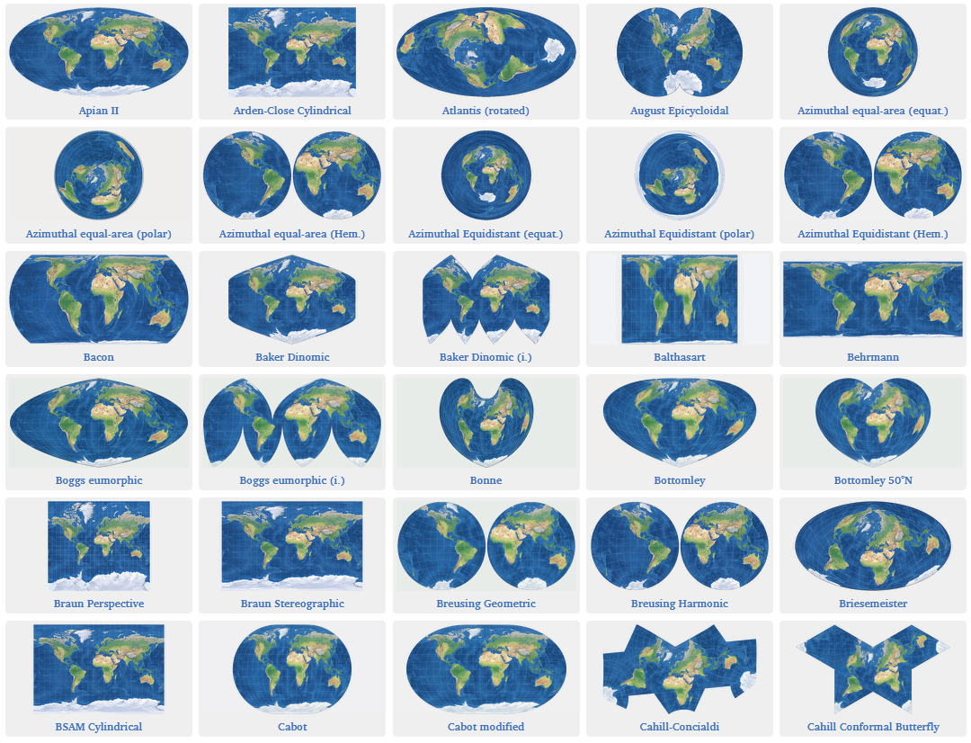
Figure 6.32: Different projections from ‘Compare Map Projections’ (map-projections.net).

The Robinson projection is an example of such a compromising projection (Figure 6.33). This pseudo-cylindrical projection was introduced in 1963, by Arthur H. Robinson. Its design is not based on mathematical formulas, but on tables in which each pair of spherical coordinates is assigned to a pair of planar coordinates. Since this planisphere gives an appealing and visually accurate image of the Earth, it is often used in atlases and in schools.

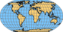
Figure 6.33: Robinson projection.

The National Geographic Society (NGS) used the Robinson projection for its world maps between 1988 and 1998. However, in 1998, NGS decided to switch to the more accurate Winkel Tripel projection (Winkel III) (Figure 6.34), which has a better ratio of shape distortion to area distortion. This resulted in a significant increase in the use of this projection during the last few years.

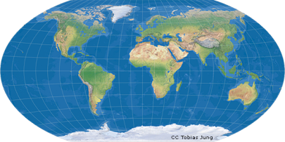
Figure 6.34: Winkel Tripel projection.

Further reading:

• Compare Map Projections - Website and Blog
• USGS “Cheatsheet” on Map Projections
• Storymap: Map Projections in ArcGIS by Bojan Šavrič & Melita Kennedy with 72 map projections (Hint: In case it does not load, you can search for the StoryMap in your web browser. Don’t forget to include the title and authors.)

6.10 Visualisation of Projection Properties

In the 19th century, the French mathematician Nicolas Auguste Tissot developed an indicator that determines the properties of a projection at one point to assess the nature and extent of geometric distortions in map designs: the Tissot indicatrix.

The Tissot indicatrix shows how an (mathematically correctly termed) infinitely small circle placed on the Earth’s surface would look like projected on a map. Since such a circle is too small to be visible on the map, its shape and size is greatly exaggerated. The size and/or shape of such a circle gets deformed due to the projection. A comparison of such deformed circles with a reference circle – the one that shows what a circle looks like when the projection properties are preserved – indicates the kind and degree of deformation at a particular point on the map.

We can also derive numerical figures from the indicatrix to quantitatively describe and compare these deformations (distortions). As the extent of geometric distortion within a projection varies locally, one must use the indicatrix at several points. This provides a good overview of the spatial variation of deformation intensity.

In Figure 6.35, Tissot indicatrices are shown on a Mollweide projection. The shape distortions clearly increase towards the edge. Since this is an equal-area projection, the true area of the indicatrix and the reference circle match at any point.

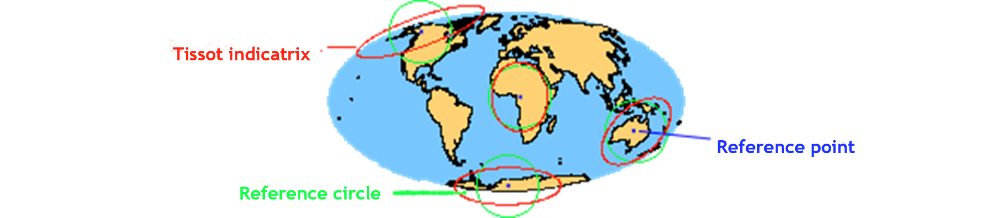
Figure 6.35: Tissot indicatrix.

Before you continue with the exercise on Tissot indicatrix, explore Esri projections and distortions visualization tool.

6.10.1 Exercise: Tissot Indicatrix

This exercise is inspired by the maps discussed in the older ArcGIS Blog Tissot´s indicatrix helps illustrate map projection distortion by Buckley (2011).

Your task is to create your own Tissot’s Indicatrix in ArcGIS and use it to explore the forms of a graticule and distortions of geometric properties for different projections.

1. Before you start

The data for this exercise is a subset of the data available in the aforementioned ArcGIS Blog (Buckley 2011) and include the following shapefiles:

• Points: locations of the intersections of the parallels and meridians of the graticule
• Admin: administrative boundaries of the world countries
• LatLog: graticule of parallels and meridians

Download and unzip this subset of the dataset here - Tissot.zip.

2. Visualise the data and identify the projection of the dataset

• Start ArcGIS Pro and create a new project.
• Open a new Map and add the 3 shapefiles.
• Your screen should look like Figure 6.36.

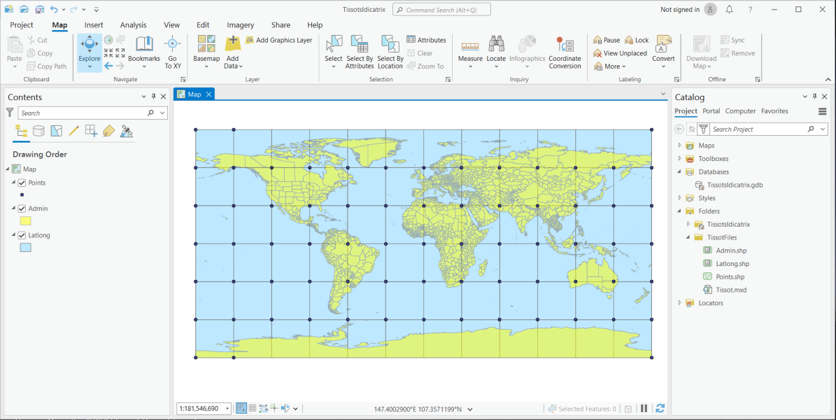
Figure 6.36: Visualise the exercise data in ArcGIS Pro.

What is the coordinate system of the map layer and of the datasets? Hint: check individual layer properties and map properties (Figure 6.37)

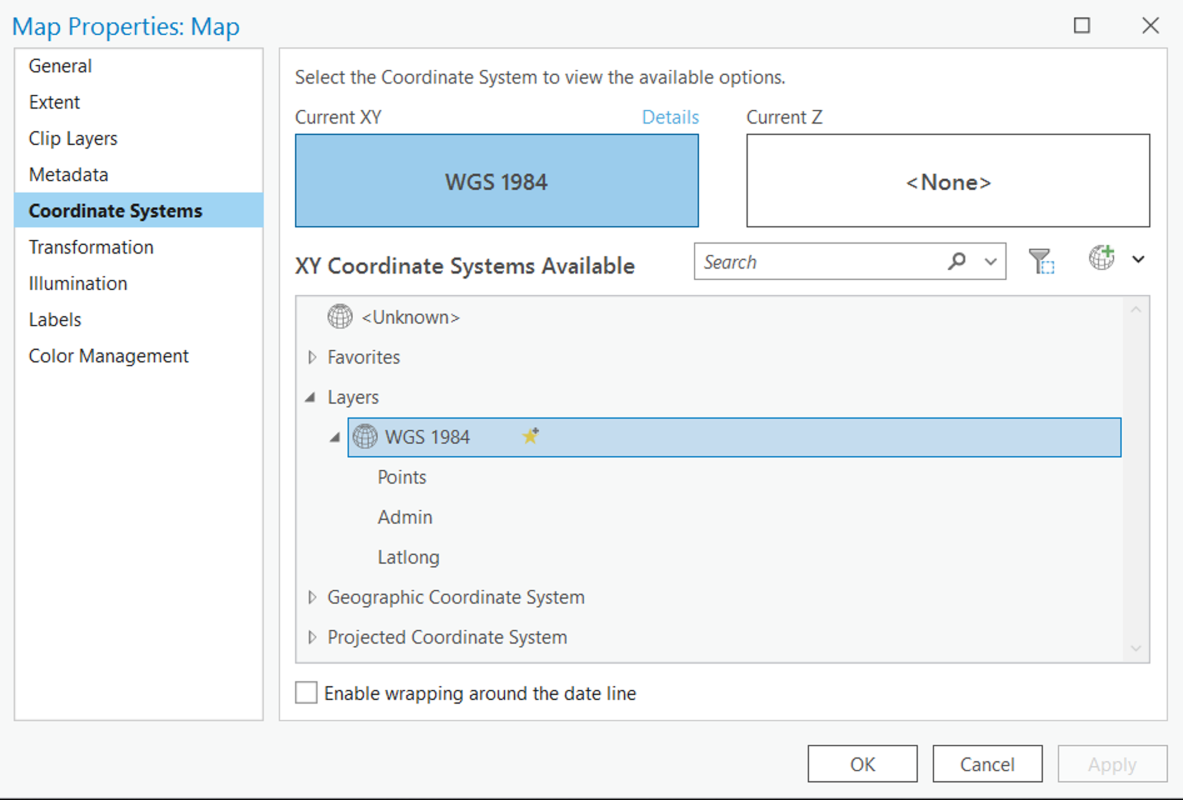
Figure 6.37: Map layer properties: info on coordinate system.

3. Create the Tissot Indicatrix

Create a 500km buffer around the points; in reality these are circles with a radius of 500km.

• Go to Analysis > Tools > Analysis Tools > Proximity > Buffer or Analysis > Tools and search for the Buffer tool the Geoprocessing Pane (Figure 6.38 - left)
• Set parameters as indicated (Figure 6.38 - middle). Store the output feature class in your project geodatabase; set the environment (Figure 6.38 - right), use the output coordinate system of the map; run the tool

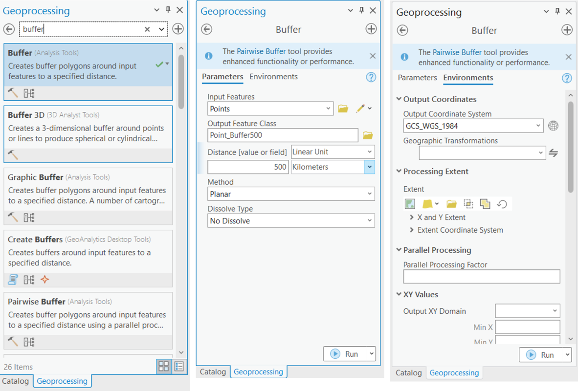
Figure 6.38: Search for the Buffer tool (left) and set the buffer parameters (middle and right) for creating the Tissot ellipsoids.

• After you run Buffer, the resulting feature class will be stored in your project geodatabase and added to the currently open Map ((Figure 6.39

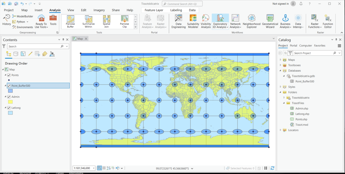
Figure 6.39: WGS 1984 - Tissot indicatrix.

Describe the pattern of distortion for the graticule and the buffers based on what you know about the properties of a given coordinate system, in this case WGS 1984 (refer to Bukley’s article for examples).

4. Explore patterns of distortion

Change a coordinate system/projection of your Map (Map > Properties > Coordinate Systems > chose a projection > Apply) and explore a resulting pattern of distortion, e.g., for the following examples:

• conformal projection – Mercator

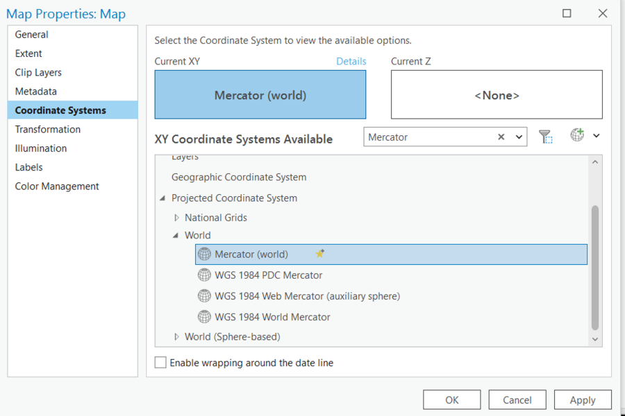
Figure 6.40: Set Mercator (world) as new projected coordinate system of the map layer.

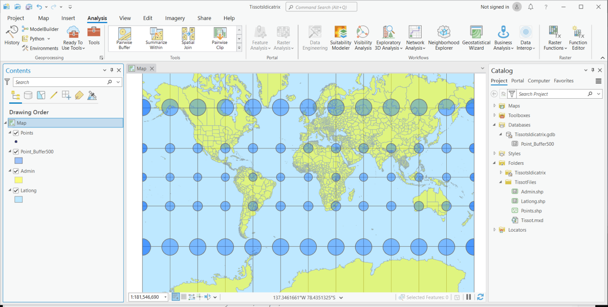
Figure 6.41: Mercator (world) - Tissot indicatrix.

• WGS 1984 Web Mercator

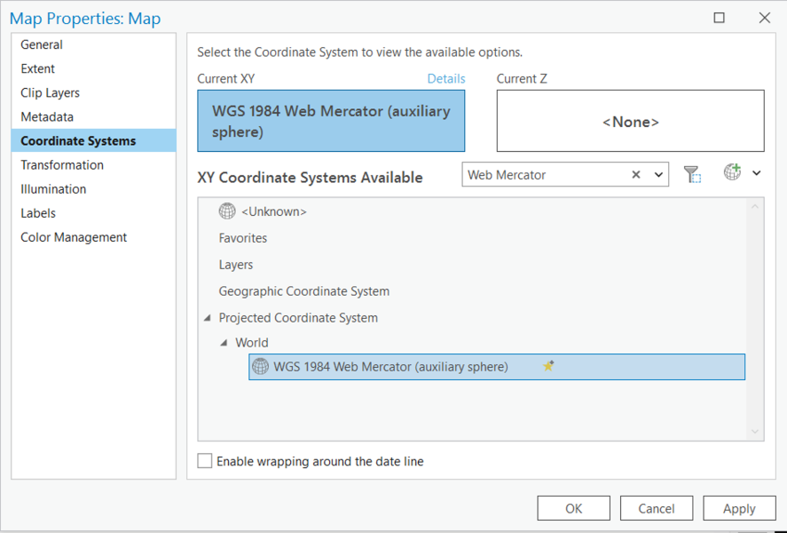
Figure 6.42: Set WGS 1984 Web Mercator as new projected coordinate system of the map layer.

How is it different from Mercator or WGS1984?

• equal area projection – Mollweide
• compromise projection - Winkel Tripel
• azimuthal equidistant
• any other…

Share your findings with your peers in the discussion forum!

6.11 Exercise: Projection parameters

To digest all the concepts of projecting the Earth’s curvature onto a flat map or screen, Figure 6.43 is an online app provided by PennState University that allows you to explore some popular map projections and settings interactively.

Figure 6.43: Explore map projections (Source: Penn State University).

Where would you set the Central Meridian, and the Standard Parallels for a Lambert Conformal Conic projection of Australia, given that Australia (without Tasmania) extends between East to West from 112°E to 153°E and from North to South between 10°S and 39°S?

Show Solution

The Central Meridian should be at the very East of the area of interest to avoid negative values. So, the Central Meridian should be set to 112°E.

The Standard Parallels should cut the Earth so that the bands above and below each of the two parallels are minimised, so we need to divide the North-South extent by four bands. The entire continent stretches over \(39° - 10° = 29°\) from North to South. So, one band should have a width of \(29° / 4 = 7.25°\). Thus, Standard Parallel 1 cuts at \(10°S + 7.25° = 17.25°S\) and Standard Parallel 2 cuts two bands further south, at \(17.25°S + 2 * 7.25° = 31.75°S\).

Set these parameters in the interactive app of Figure 6.43 and update the map. Does the map projection meet your expectation?

6.12 Quizzes

In Quiz 6.44 match the map projections with the correct explanation. Check, whether your solution is correct by clicking on the blue checkbox icon in the bottom right corner.

Figure 6.44: Quiz: Match the projections with its definition.

Finally, find the correct answer in Quiz 6.45. Check, whether your solution is correct by clicking on the blue checkbox icon in the bottom right corner.

Figure 6.45: Quiz - least distortion.

6.13 Summary

In this lesson, we discussed the projections, i.e., the geometrical transformation of the curved (ellipsoidal or spherical) surface of the Earth onto a flat map surface. We looked into various types of projections based on, e.g., developing surface, aspect, or geometrical properties they can preserve. An understanding of projections is essential to understand “international relations in our global society” (Kimerling et al. 2016).

Criteria for choosing a projection

After all the discussion on projections, the choice of a suitable one should no longer be an unsolvable problem; here are a few considerations that are important when choosing an appropriate projection:

• Existing reference systems

  In many GIS projects, the question of the best projection to be used is often irrelevant because it has already been specified by the client. It makes perfect sense to use the “official” spatial reference systems or standards such as UTM in continental scale maps.

• Primary application area of the map

  The geometric properties to be preserved depend upon the purpose of the actual map representation:

  • The distribution or dissemination of a phenomenon is preferably presented in a projection that preserves the area.
  • Maps for navigational purposes will use conformal, equal-area and/or equidistant projections.
  • General overview maps at a medium scale mostly use angle preserving projections.
  • Pseudo projections are best suited for world maps that are expected to provide a realistic representation of the Earth as a whole.

• Size of the area to be projected

  The differences between various map projections become increasingly obvious the further we move away from a point or line of tangency. Therefore, the decision for a particular projection is more critical if a larger area needs to be covered.

• Location of the area to be projected

  Primarily for medium- and small-scale maps, the following rule of thumb results from how the projection surface fits the body of the Earth:

  • Azimuthal projections for polar regions
  • Conic projections for projecting regions near / in the mid-degrees of latitude
  • Cylindrical projections for equatorial areas

• Shape of the area to be projected

  The shape of the area to be projected is only significant in medium- and small-scale maps:

  • Azimuthal projections for more compact shapes
  • Conical or cylindrical projections in areas with a large east-west extent
  • Transverse cylindrical projections in narrow areas with a large north-south extent

6.13.1 Video on Projections and Coordinate Systems in GIS

In the following video, you can watch a summary on projections and coordinate systems produced by Dr. Gudrun Wallentin and Dr. Christoph Traun, in 2023:

Figure 6.46: Video (24:45) UNIGIS Talks ep. 1: Projections and Coordinate Systems in GIS.

6.14 Assignment: Working with Coordinate Reference Systems and Projections

Now, it is time for the next assignment. For further instructions, please switch to Moodle.

References

Buckley, Aileen. 2011. “Tissot’s Indicatrix Helps Illustrate Map Projection Distortion.” ArcGIS Blog https://www.esri.com/arcgis-blog/products/mapping/mapping/tissots-indicatrix-helps-illustrate-map-projection-distortion/.

Kimerling, A Jon, Aileen R Buckley, Phillip C Muehrcke, and Juliana O Muehrcke. 2016. Map Use: Reading, Analysis, Interpretation. Esri Press Redlands, CA.