Lesson 3 Geoinformatics in Action
Geoinformatics applications are found in a wide range of fields. Increasingly, they are no longer stand-alone mapping applications, but apps and tools built into websites, devices, and machines. Understanding the science behind the applications will help you to understand how Geoinformatics has been integrated into the decision-making processes of our everyday lives.
In this lesson, we consider multiple case studies and applications across a range of disciplines. This should be an appetiser for you to start your own exploration of the world of Geoinformatics in action.
There is a wide variety of projects that benefit from the perspective brought by geospatial professionals. When we look more closely at examples of these case studies, we can often relate them to one of the following domains:
- Government
- Transportation and Logistics
- Utilities
- Natural Resources
- Business
- Health
What other disciplines can you think of? If you think about it, you will probably find it easy to add a few disciplines, starting somewhere with “A” like in Archaeology, and ending with disciplines with “Z” like in Zoology.
Upon completion of this lesson, you should be able to:
- Provide examples of current applications in Geoinformatics
- Identify where geospatial intelligence is embedded
- Describe projects that can benefit from spatial data handling and analysis
- Identify the power of GI-Systems in problem solving
3.1 Emergency and Disaster Management
Disaster Management puts the focus on human well-being and its relation to the environment in case some extraordinary events happen. It defines spatial relations based on data like distance, speed, neighbourhoods, and it can be essential for analysing and predicting disaster events, as well as for decisions for best-reaction-scenarios in an emergency.
GI-Systems analyse past events systematically to create models capable of predicting future events. Based on these regularities, probabilities can be calculated. As an example, we can “feed” a model with data about topography, soil moisture, soil structure, and vegetation to predict landslides with regards to different intensities of rainfall.
In the event of an emergency, time is a key factor. GIS offers a possibility to connect to sensors, to show “real-time-data” and to further provide high quality information to the people involved. GIS also plays a big role in answering the two main questions “What is where?” and “Where is what?” for evacuation and rescue measures. By combining inventory data (e.g., road maps) with real-time data (e.g., sensor data like traffic counts) and remote sensing data (e.g., post-event images) the information base for taking lifesaving actions can be provided within short time.
This demonstrates the power of GIS. Based on this potential, the United Nations (UNO) have created the UN-Spider portal collecting space-based information for disaster management: UN Spider portal
For exploration and further reading, take a look at some selected examples where GIS is used for Emergency and Disaster Management:
- National Geographic: Amazon fires
- The Refugee Project
- Earthquake Hazards Program by USGS (Figure 3.1)
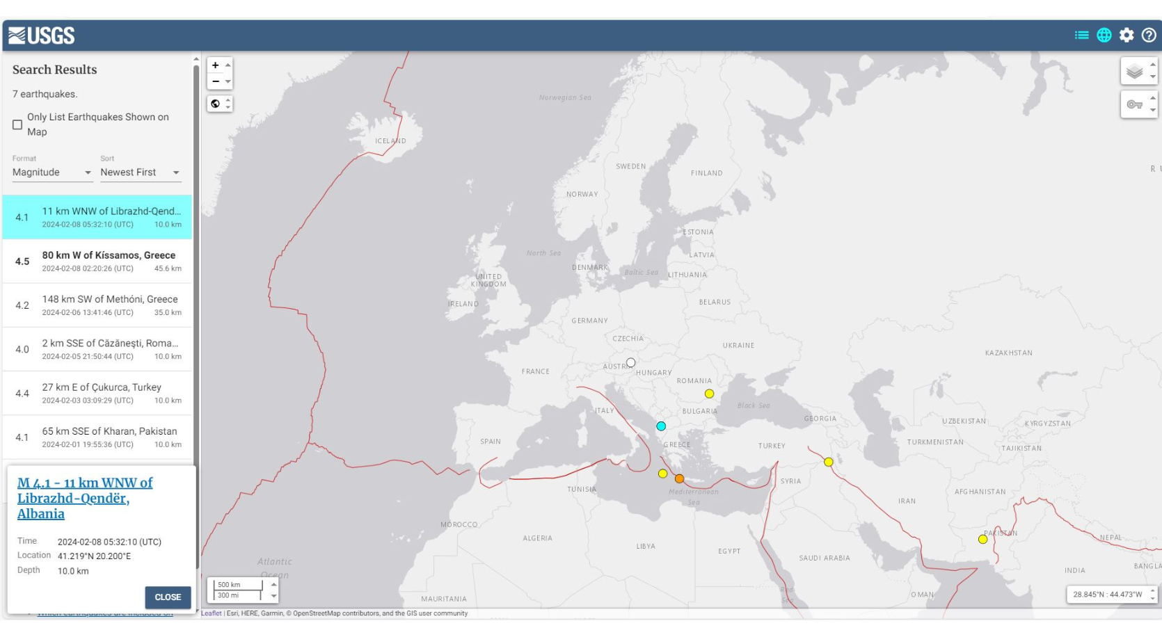
Figure 3.1: USGS Earthquake Monitor (Screenshot)
3.2 Climate Change and Health
Climate change and the resulting implications increasingly influence human health. While people in wealthy parts of the world find ways to cope with the changes, people in low-income areas are extremely vulnerable and powerless against the changing environmental conditions. Vector-borne diseases spread easiest along water bodies, which are very much affected by climate change, as vectors are mostly water-bound mosquitos or ticks. Based on the model data, direct (further infections) and indirect consequences (food shortages or contamination of life stock) can be prevented. These analyses facilitate organising help in emergency situations and optimising prevention measures.
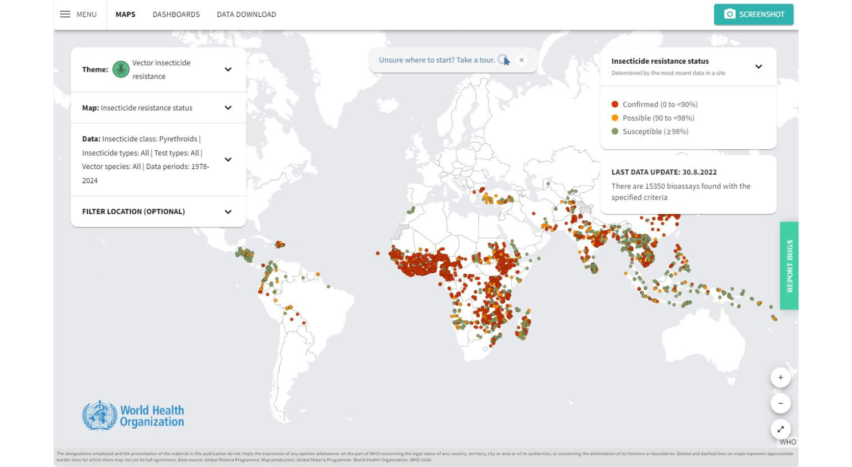
Figure 3.2: Malaria Risk Map (Screenshot).
The WHOs interactive website Vector insecticide resistance demonstrates the application possibilities for using spatial models as shown in Figure 3.2.
3.3 Spatial Planning
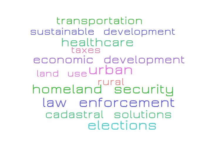
Figure 3.3: Governmental GIS Tasks.
Governments and, especially, local governments are one of the major users of GIS (Figure 3.3), mostly because 70-80% of local government tasks are geographically related. Due to the constantly increasing utilisation of space and resulting land-use conflicts, the use of computerised workflows is inevitable. GI-Systems often play a key role in organising municipal data.
One main task is land-use management containing a large number of data layers, e.g., land registry, graveyards, playgrounds, protected areas, land-use plan, electricity and water supply networks, sewer, roads, schools, fire brigades etc. Spatial databases help in connecting and selecting layers and extracting the relevant information for given tasks. Web-based GIS solutions pave the way for civic participation in planning, by establishing a communication platform, on which scenarios can be drawn and commented.
One very fine example of an interactive City GIS is provided by the City of London; a screenshot is shown in Figure 3.4.
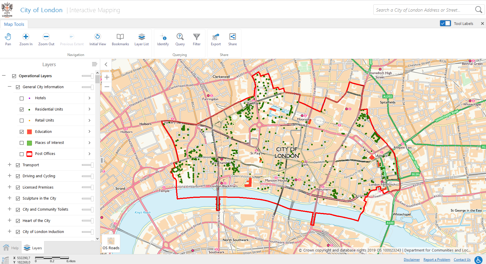
Figure 3.4: City of London Interactive Mapping.
For further reading:
- an excellent example can be found at the Alberta Geological Survey website. Explore the interactive maps!
- Hazards mapping, history and the future of Rust Belt cities.
- Siting a Low-Level-Radioactive Waste Disposal Facility in New York State - A Case Study in the Misuse of GIS by Mark Monmonier. He is known for his still thought-provoking book “How to Lie with Maps”, in which he promotes “a healthy scepticism about maps” (Monmonier 2005).
3.4 Transportation and supply networks
Transportation and logistics are amongst the traditional areas of GIS applications. They deal with the movement of people and goods between places and with the infrastructure that moves them. Operators of supply networks (water, gas, electricity, sewer, telecommunication etc.) have a lot in common with the transportation industry - both use networks as ways for transporting their goods. Have a look at Figure 3.5 of the gas supply network of Ireland, this map can be inspected in greater detail at gas networks.
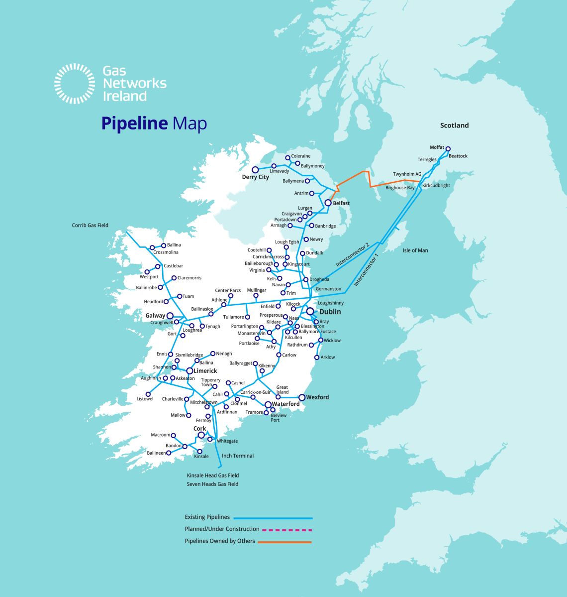
Figure 3.5: Gas supply network in Ireland (Source: Gas Networks Ireland).
Highway authorities, for example, need to know the amount of traffic on individual roads to be able to prevent congestion through a near-real-time redirection of the traffic (operational applications). In the long term, they also need to plan and build new roads (strategic application). Delivery or service companies need to organise their fleet in a way that all pick-up and delivery locations are serviced with a minimum loss of time, e.g., time spent in unnecessary driving.
The majority of tasks included in operational and tactical applications are based on network analysis (e.g., shortest-path methods), scheduling, and they involve a great deal of optimisation. Functions further needed from a GIS are used to create, manage, and visualise information about networks. In all these cases, the information produced is used to support decision making. The oldest examples of a highly sophisticated use of transportation and logistics applications are found in the military.
3.4.1 Optimising the Transportation of Goods
Countless software products offer route optimisation and site selection based on digital road networks. They also provide short term reactions to:
- driving speed,
- road condition and congestion,
- border crossings, and
- short term blockages.
These applications increase efficiency and reduce the costs for enterprises.
Figure 3.6: ESRI StoryMap about Optimising Home Delivery.
3.4.2 Mobility Research
Movement and the transport of people and goods are spatial by their very nature. Thus, spatial computation and mobility research have been converging over the last few years. In this context, two innovative fields have emerged in recent years:
- Data modelling
Modelling movement and tracking data is difficult because of its spatial and temporal characteristics. New types of data models and database designs enable an increased computing performance.
- Availability of data
Mobile devices have a multitude of sensors integrated, including a GPS. Digital traces of mobile phones, combined with steadily growing open infrastructure data, deliver vast amounts of data in real-time which can be used by mobility researchers.
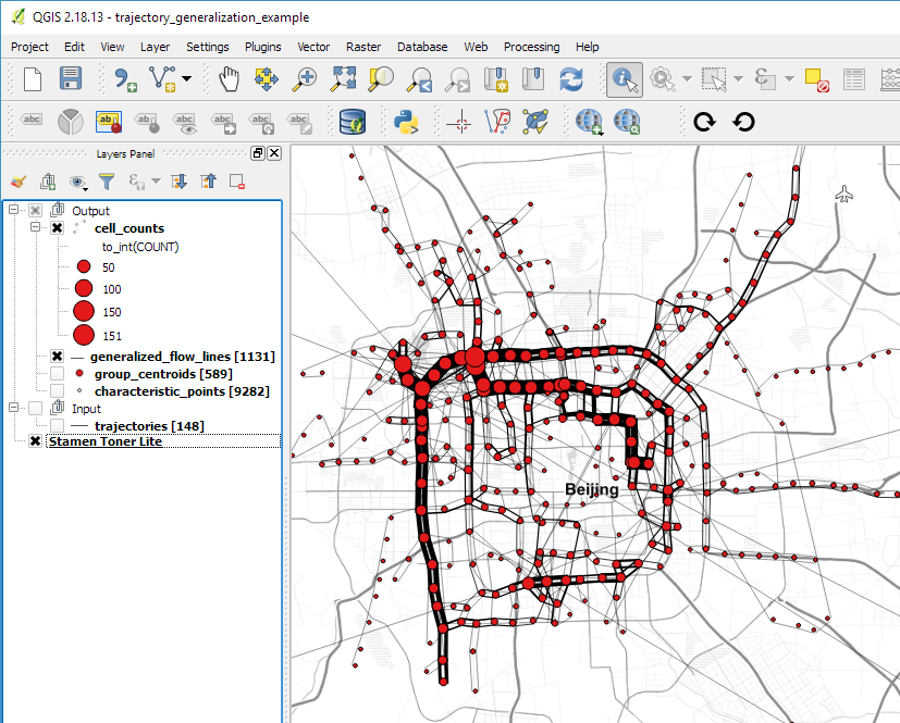
Figure 3.7: Trajectory generalisation from movement data. Blog by Anita Graser (see below).
For further reading and exploring:
- GIS Movement data blog by Anita Graser
- Mapnificent shows how far you get by using public transport within a given time
- Flightradar24.com
- Marinetraffic.com
- GIS and Transport Modelling - “Strengthening the Spatial Perspective”
3.5 Business Geography
The term “Business Geography” implicates terms like:
- Marketing and market research
- Site selection
- Locating profitable markets
- Locating untapped market areas and emerging markets
- Performing effective target marketing (geo-marketing)
- Analysing market penetration
- Visualising consumer expenditure data, etc.
GIS has been applied at all scales
- Operational – processing day-to-day transactions (e.g., delivery vehicle routing)
- Tactical – allocation of resources to short-term (weekly) problems (e.g., target marketing promotional campaigns)
- Strategical – long term goals and missions (e.g., store location planning)
In addition to the notes above, business and service planning GIS comprise financial services, insurance, and real estate. Most business applications are either operational, tactical, or strategical in nature. The expected benefits range from quantifiable and measurable economic benefits (e.g., increase in sold products, saving of money or time, etc.) to benefits like increased accuracy, efficiency, and productivity, or reduction of workload, decision support, and resources management.
For further reading:
- Pinpoint by Foursquare - location based marketing
- Article in MarketingTechNews - “Why location data matters - even if you’re not a retailer”
- Indoor-Atlas a Finnish enterprise targeting the problem of indoor navigation
3.5.1 Consumer Behaviour
Geoinformation technology can be used to study consumer behaviour, which is decisive to a business setup. Fashion retailing, for example, is one type of business that relies heavily on the walking behaviour of consumers. Retailers are often concerned with a truly profitable location for their stores, which simply means a location with a high pedestrian flow.
A shopping plaza is an ideal testing place for consumers as most people are going there for shopping. With the construction of many large shopping plazas worldwide in recent years and, especially, in dense urban cities, it is highly beneficial to know why some locations are frequently visited or passed by shoppers.
The walking routes of shoppers within the plazas can be recorded and stored in a GIS and the routing pattern can be modelled. Frequently visited routes can be derived and by correlating the pattern with a set of environmental or spatial variables, and with non-spatial variables like degree of familiarity, demographic factors, a shoppers’ preferences and, in particular, their habitual walking patterns, they can be more thoroughly researched (Pun-Cheng and Chu 2004).
3.6 Archaeology
Since Archaeology is a spatial science too, GI-Systems are highly appropriate tools to capture, store, manipulate, analyse, and display archaeological data.
Geographic Information Systems (GIS) and related remote sensing technologies offer powerful means of analysing water flow and are well-suited to clarify design and operational requirements of different irrigation and water management systems. Ancient Southwest Arabian irrigation technologies developed over thousands of years, culminating in some of the ancient world’s most advanced flash-flood and irrigation water systems.
Standford University created Orbis - a “routing system” for the Roman Empire taking into account communication costs in terms of both time and expense. By using the Roman road network, main navigable rivers, and hundreds of sea routes, this interactive model reconstructs the duration and financial cost of travel in antiquity.
Further reading on Archaeology and GIS:
- Uncovering the past using the future: How lasers are revolutionizing archaeology
- 3D GIS for cultural heritage restoration: A ‘white box’ workflow (paper on 3D GIS in Pompeii)
- PASTMAP - Historic Environment Scotland (mind the zoom level for the data layers)
- Vici Map: Archaeological Atlas of Antiquity - open-source project to map antique sites
3.7 Ecology and Nature Conservation
Our everyday life is inevitably linked to using natural resources. To avoid negative effects, this must be done in the most effective way possible. To use the limited resources with consideration, geospatial applications are used for documentation as well as for analytical, and modelling purposes.
Nature conservation aims at protecting biotic and abiotic resources and their functional relationships. GI-Systems play an important role for gathering and illustrating the status, as well as for monitoring changes over time, and for modelling future developments. An example is demonstrated in the video in Figure 3.8.
Figure 3.8: VIDEO (3:10) Worldwide CO2 change over 1 year.
Open Government Data (OGD) have become an indispensable backbone for nature conservation projects. Exemplary platforms for environmental data are the London Datastore, or Open Data Österreich for Austria.
3.7.1 Environmental Information System
Environmental Information Systems (EIS) are maintained by governmental institutions or for specific domain applications. The boundaries do not necessarily need to be country boundaries, they can also consider, for example, habitats or geographical regions. Environmental Information Systems can contain “hard facts” like soil contamination with a certain substance and “soft facts”, e.g., laws, reports, or evaluations.
The purpose of EIS is to grant access to environmental information for a broader audience (see Figure 3.9) to facilitate resource-efficient planning and to ensure transparency in law enforcement, e.g., make causes for new laws accessible.
Figure 3.9: Half-Earth Project Map (by E.O. Wilson Biodiversity Foundation). Scroll down and explore the maps and data.
Click here to get to the interactive map. Select between Priority Areas and National Report Cards.
For further reading:
3.7.2 Species Distribution Models
Species distribution models make use of species observation data and environmental data layers to model the potential distribution of plant or animal species. These models consider all the layers of spatial information that are relevant for a specific species, e.g., elevation, slope, climate, land-use, water temperature, or ocean currents. By extracting typical local characteristics, a set of conditions can be created, the so-called “ecological niche” of a species. The set of conditions describing the ecological niche can then be used to map the potential occurrence of the examined species.
Figure 3.10: Swiss Topic Center on fauna. Try it out and search for a species, e.g., type in ‘butterfly’. Hint: You can set the language to English in the upper right corner.
At the Swiss Topic Center on Fauna many species distribution maps can be explored as shown in Figure 3.10. Go to Map Server CSCF for a full screen view.
3.8 Exercise: Tree Cadastre of Linz
This exercise will prepare you for the assignment of this lesson, in which you will do hands-on analysis with spatial data. The methodological approach in this exercise is similar to what you are going to do in the Assignment 2. Exercises are particularly well suited for asking questions of methodological nature as well as for getting familiar with the software.
Trees have an important and notably positive influence on environments in urban areas. Apart from reducing CO2, they provide shade and help to cool the air. Having many trees and knowing where they are, can be a valuable location factor. Further, a tree cadastre is important for the urban government to take care of the green lung of their city.
In this exercise, we will work with Open Governmental Data (OGD) for the city of Linz (a town in Austria) to show how data can be turned into valuable information by using Geoinformatics. Before starting this, Assignment 1 should be completed, and you should have accustomed to working in Esri ArcGIS Pro. In this exercise, you will work with data in a feature layer that needs to be saved locally.
Step 1
Open a new Map in ArcGIS Pro and search for the online dataset “UNIGIS Exercise tree cadastre”, which is hosted on ArcGIS online: in ArcGIS Pro > open Catalog > Portal > ArcGIS online (cloud symbol) > use the search field > add to current map.
The tree locations show only the trees on public land, which are taken care for by the local administration. To get information about the density of these trees, it is necessary to aggregate the tree locations to spatial reference units. Therefore, we implement two polygon grids with two different grid sizes.
Step 2
Search the ArcGIS Toolkit Analysis > Tools > Geoprocessing pane opens > for Create Fishnet and open this tool (Figure 3.11). Choose the following parameters:
- Output Feature Class = fishnet500
- Template Extent = project area (select the layer icon and chose the layer “UNIGIS Exercise tree cadastre_area”)
- Cell size width = 500
- Cell size height = 500
- Create label points = unchecked
- Geometry type = polygon
Run
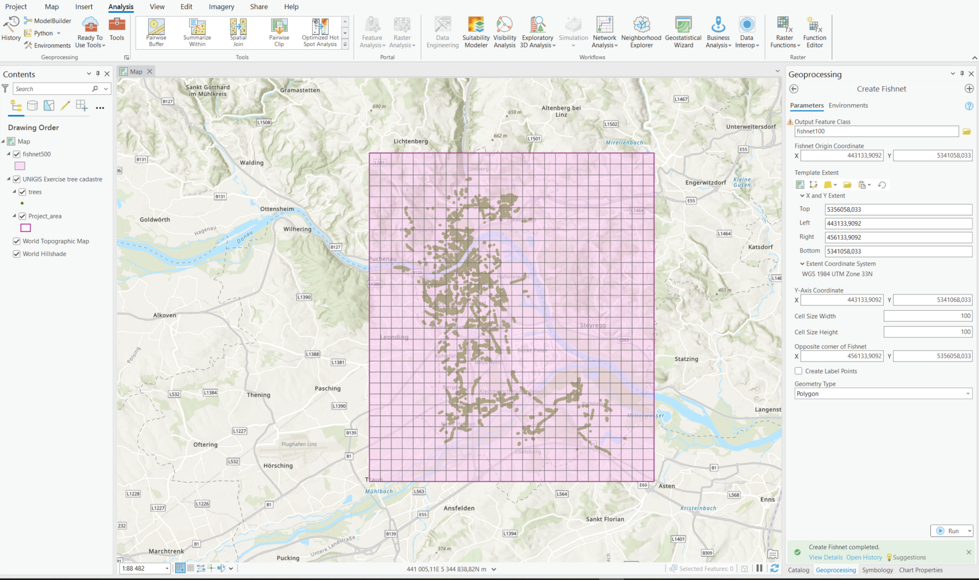
Figure 3.11: Parameters for creating the fishnet (right) and the resulting fishnet (middle), ex. 500x500, with minor transparency changes to see the trees.
Step 3
Create a second grid covering the project area with a cell size of 100x100m. The result should look like Figure 3.12 below.
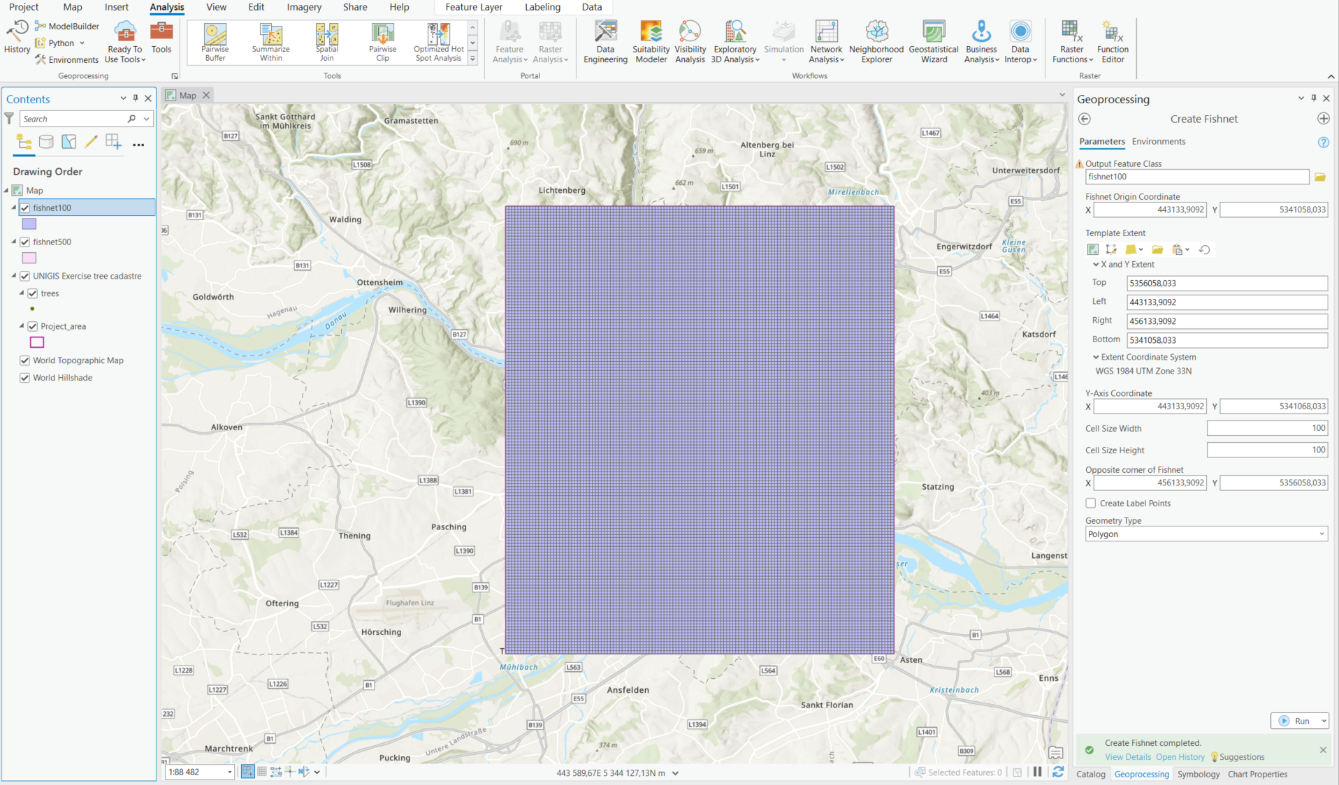
Figure 3.12: Parameters for creating the fishnet (right) and the resulting fishnet (middle), ex. 100x100.
To calculate the density of trees, the tree locations must be spatially joined with the reference areas. There are various methods how to conduct such a join (= match option). In this exercise, we use intersect, but contains can also work. This means that the tool is looking for all trees that intersect with certain areas. Have a closer look at the match options in Step 4. Always be aware of what the “Target Feature” and what the “Join Feature” is. Try to switch them to see what happens. To see how the size of the reference area influences the result, we will do this step for both grid sizes.
Step 4
Open the tool Spatial Join in the Geoprocessing toolkit and parameterise it like this:
- Target Features = Fishnet500
- Join Features = trees
- Join Operation = Join one to one
- Keep all Target Features = checked
- Match Option = Intersect
- Search Radium = leave empty
Run
The field “Joint Count” will be created and filled in automatically. The value shows the number of tree locations in each cell.
Step 5
Repeat Step 4 using the grid with cell size 100.
Step 6
Create two maps showing the density with respect to the grids 100 and 500. You can exclude the cells without tree location from being displayed. One way of doing this is a definition query (right mouse click on the selected Layer > Properties > Definition Query) with the argument 'Join Count > 0' > Apply.
The maps should look as shown in Figures 3.13 and 3.14:
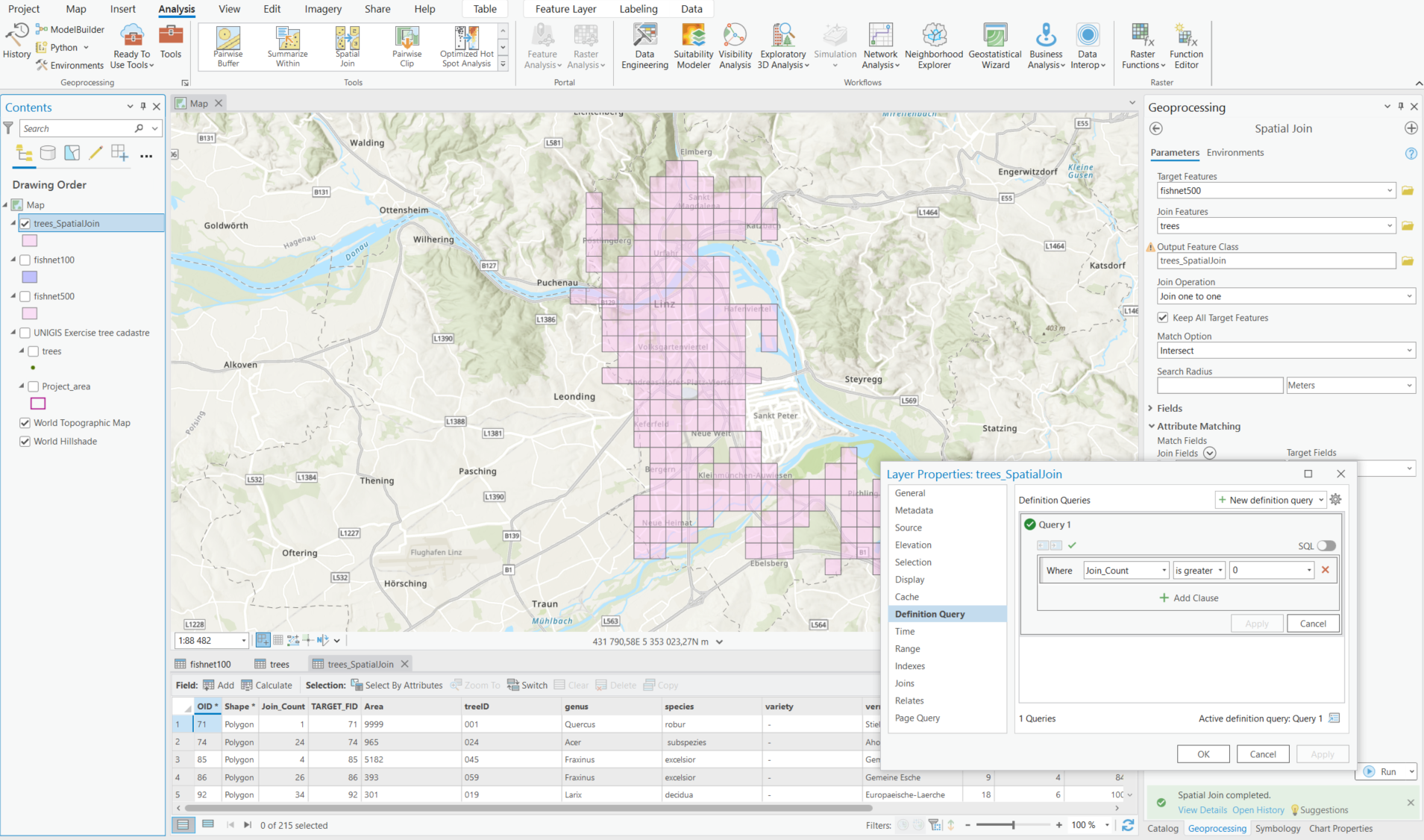
Figure 3.13: Result: 500x500 after definition query.
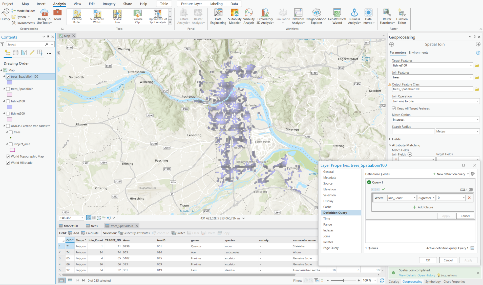
Figure 3.14: Result: 100x100 after definition query.
If you want to know some statistics about the distribution of the trees, open the Attribute Table of the layer (right click on Layer > Attribute Table) and look for the “Join_Count” entries. With another right click on the head of the column, e.g., Join_Count, you can activate the statistics.
Step 7
Answer the following questions and post them in the discussion forum on Moodle:
- How can the spatial distribution of tree locations be described verbally?
- How do the spatial patterns in density change between the different spatial reference areas?
- For which spatial analysis is the aggregation level a key factor? Please refer to specific use cases.